Google Capstone Project: Bellabeat 🏃♀️
Introduction
As part of the Google Data Analytics Professional Certificate, this was the second optional case study provided. I have chosen to also do this project in order to enhance and reinforce my new skills. Like the previous project, this project will outline the following processes as taught in the programme; Ask, Prepare, Process, Analyse, Share and Act. To clean and manipulate the data, R programming will be used due to its vast efficiency. Unlike my previous Capstone Project, R programming will also be used for the visualisations.
Scenario
Bellabeat is a high tech manufacturer of health focused products for women. Although it is a small and successful company, Bellabeat has the potential to become a larger player in the global smart device market. Urška Sršen, the cofounder and Chief Creative Officer, believes new growth opportunities can be unlocked for the company by analysing the smart device fitness data. Therefore, the data analytics team wants to analyse one of their products in order to discover how consumers are using their smart devices. These insights will then guide and improve the current marketing strategy.
About the company
Established in 2013, cofounders Urška Sršen and Sando Mur have made Bellabeat a growing success and rapidly positioned the company as a tech-driven wellness company for women. Sršen expertise has allowed the development of an appealing designed technology that informs and inspires women around the world by tracking data on their activity, sleep, stress and reproductive health.
The marketing team have been asked to focus on a Bellabeat product and analyse its smart device usage to gain insights into how people are using it. This information will then allow a high level recommendation for how these trends can enhance Bellabeat’s marketing strategy and reveal more growth opportunities.
Business Task
Analyse one of the company’s products and explore the smart device data to gain insight into how customers use non-Bellabeat smart devices.
Product
Bellabeat app: The app provides users with health data related to their activity, sleep, stress, menstrual cycle, and mindfulness habits. This data helps users better understand their current habits and make healthier decisions. The app also connects to their line of smart wellness products.
Stakeholders
- Urška Sršen: Bellabeat’s cofounder and Chief Creative Officer
- Sando Mur: Mathematician and Bellabeat’s cofounder; key member of the company’s executive team
- Bellabeat’s marketing analytics team: A team of data analysts responsible for collecting, analysing and reporting data that helps guide Bellabeat’s marketing strategy
Ask
The following three questions will guide the analysis:
- What are some trends in smart device usage?
- How could these trends apply to Bellabeat customers?
- How could these trends help influence Bellabeat marketing strategy?
Prepare
The data used in this project was the FitBit Fitness Tracker Data (CC0: Public Domain, data set made available through Mobius). The data set was created by respondents to a survey distributed on Amazon Mechanical Turk and corresponded to the period between 12.03.2016 and 12.05.2016. It explores smart device users’ daily habits and contains personal fitness tracker from thirty FitBit users. These users consented to the submission of their personal tracker data that consists of their minute level output for physical activity, heart rate, and sleep. There is a variation between output as it represents the different types of FitBit trackers used and personalised tracking preferences.
Data organisation
Eighteen CSV files are zipped into the data set and incorporates specific tracking information such as, daily calories, daily steps, activity intensity etc. It is organised in a long format whereby an ID column identifies each user, whilst the rest focuses on the attributes about the user.
Data integrity
Considering the sample size of the data set of only 33 FitBit users and 2 months worth of information, it is important to note that the data is not a complete representation of all FitBit users. In addition the data set is from seven years ago, thus users preferences and habits may have changed. Overall, this is potential credibility bias due to the aforementioned reasons as well as the data being collected by another party.
Despite this, the analysis will still continue and discover insightful information regarding the surveyed users and how they made use of their tracking devices over the period of time.
Data security
As the data set is from an open source public platform on Kaggle it is said to have little integrity. To address the privacy and security the data is anonymised with no personal identifiable information in the data. Instead it is classified with the use of unique IDs which linked to the different data set.
Load required R packages
library(tidyverse)
library(lubridate)
library(janitor)
library(skimr)
library(readr)
library(dplyr)
library(tidyr)
library(data.table)
library(ggpubr)
library(ggrepel)
Import and load the data sets
daily_activity <- read.csv("~/Documents/Bellabeat_Capstone/ dailyActivity_merged.csv")
daily_sleep <- read.csv("~/Documents/Bellabeat_Capstone/ sleepDay_merged.csv")
hourly_steps <- read.csv("~/Documents/Bellabeat_Capstone/ hourlySteps_merged.csv")
Console output from loading data sets
> daily_activity <- read_csv("~/Documents/Bellabeat_Capstone/dailyActivity_merged.csv")
Rows: 940 Columns: 15
── Column specification ───────────────────────────────────────────────────────────────────────────────────────────────────────────────────
Delimiter: ","
chr  (1): ActivityDate
dbl (14): Id, TotalSteps, TotalDistance, TrackerDistance, LoggedActivitiesDistance, VeryActiveDistance, ModeratelyActiveDistance, Light...

ℹ Use `spec()` to retrieve the full column specification for this data.
ℹ Specify the column types or set `show_col_types = FALSE` to quiet this message.

> daily_sleep <- read_csv("~/Documents/Bellabeat_Capstone/sleepDay_merged.csv")
Rows: 413 Columns: 5
── Column specification ───────────────────────────────────────────────────────────────────────────────────────────────────────────────────
Delimiter: ","
chr (1): SleepDay
dbl (4): Id, TotalSleepRecords, TotalMinutesAsleep, TotalTimeInBed

ℹ Use `spec()` to retrieve the full column specification for this data.
ℹ Specify the column types or set `show_col_types = FALSE` to quiet this message.

> hourly_steps <- read_csv("~/Documents/Bellabeat_Capstone/hourlySteps_merged.csv")
Rows: 22099 Columns: 3
── Column specification ───────────────────────────────────────────────────────────────────────────────────────────────────────────────────
Delimiter: ","
chr (1): ActivityHour
dbl (2): Id, StepTotal

ℹ Use `spec()` to retrieve the full column specification for this data.
ℹ Specify the column types or set `show_col_types = FALSE` to quiet this message.
Prepare
To process the data sets, R programming language will be used. In this section the data will be cleaned and manipulated for analysis.
Identify and view data set using functions
head(daily_activity)
Console output
# A tibble: 6 × 15
          **Id ActivityDate TotalSteps TotalDistance TrackerDistance LoggedActivitiesDistance VeryActiveDistance ModeratelyActiveD…¹ Light…² Seden…³ VeryA…⁴ Fairl…⁵ Light…⁶ Seden…⁷ Calor…⁸**
       <dbl> <chr>             <dbl>         <dbl>           <dbl>                    <dbl>              <dbl>               <dbl>   <dbl>   <dbl>   <dbl>   <dbl>   <dbl>   <dbl>   <dbl>
1 1503960366 4/12/2016         13162          8.5             8.5                         0               1.88               0.550    6.06       0      25      13     328     728    1985
2 1503960366 4/13/2016         10735          6.97            6.97                        0               1.57               0.690    4.71       0      21      19     217     776    1797
3 1503960366 4/14/2016         10460          6.74            6.74                        0               2.44               0.400    3.91       0      30      11     181    1218    1776
4 1503960366 4/15/2016          9762          6.28            6.28                        0               2.14               1.26     2.83       0      29      34     209     726    1745
5 1503960366 4/16/2016         12669          8.16            8.16                        0               2.71               0.410    5.04       0      36      10     221     773    1863
6 1503960366 4/17/2016          9705          6.48            6.48                        0               3.19               0.780    2.51       0      38      20     164     539    1728
# … with abbreviated variable names ¹ModeratelyActiveDistance, ²LightActiveDistance, ³SedentaryActiveDistance, ⁴VeryActiveMinutes, ⁵FairlyActiveMinutes, ⁶LightlyActiveMinutes,
#   ⁷SedentaryMinutes, ⁸Calories
str(daily_activity)
Console output
spc_tbl_ [940 × 15] (S3: spec_tbl_df/tbl_df/tbl/data.frame)
 $ Id                      : num [1:940] 1.5e+09 1.5e+09 1.5e+09 1.5e+09 1.5e+09 ...
 $ ActivityDate            : chr [1:940] "4/12/2016" "4/13/2016" "4/14/2016" "4/15/2016" ...
 $ TotalSteps              : num [1:940] 13162 10735 10460 9762 12669 ...
 $ TotalDistance           : num [1:940] 8.5 6.97 6.74 6.28 8.16 ...
 $ TrackerDistance         : num [1:940] 8.5 6.97 6.74 6.28 8.16 ...
 $ LoggedActivitiesDistance: num [1:940] 0 0 0 0 0 0 0 0 0 0 ...
 $ VeryActiveDistance      : num [1:940] 1.88 1.57 2.44 2.14 2.71 ...
 $ ModeratelyActiveDistance: num [1:940] 0.55 0.69 0.4 1.26 0.41 ...
 $ LightActiveDistance     : num [1:940] 6.06 4.71 3.91 2.83 5.04 ...
 $ SedentaryActiveDistance : num [1:940] 0 0 0 0 0 0 0 0 0 0 ...
 $ VeryActiveMinutes       : num [1:940] 25 21 30 29 36 38 42 50 28 19 ...
 $ FairlyActiveMinutes     : num [1:940] 13 19 11 34 10 20 16 31 12 8 ...
 $ LightlyActiveMinutes    : num [1:940] 328 217 181 209 221 164 233 264 205 211 ...
 $ SedentaryMinutes        : num [1:940] 728 776 1218 726 773 ...
 $ Calories                : num [1:940] 1985 1797 1776 1745 1863 ...
 - attr(*, "spec")=
  .. cols(
  ..   Id = col_double(),
  ..   ActivityDate = col_character(),
  ..   TotalSteps = col_double(),
  ..   TotalDistance = col_double(),
  ..   TrackerDistance = col_double(),
  ..   LoggedActivitiesDistance = col_double(),
  ..   VeryActiveDistance = col_double(),
  ..   ModeratelyActiveDistance = col_double(),
  ..   LightActiveDistance = col_double(),
  ..   SedentaryActiveDistance = col_double(),
  ..   VeryActiveMinutes = col_double(),
  ..   FairlyActiveMinutes = col_double(),
  ..   LightlyActiveMinutes = col_double(),
  ..   SedentaryMinutes = col_double(),
  ..   Calories = col_double()
  .. )
 - attr(*, "problems")=<externalptr>
head(daily_sleep)
Console output
# A tibble: 6 × 5
					**Id SleepDay              TotalSleepRecords TotalMinutesAsleep TotalTimeInBed**
			 <dbl> <chr>                             <dbl>              <dbl>          <dbl>
1 1503960366 4/12/2016 12:00:00 AM                 1                327            346
2 1503960366 4/13/2016 12:00:00 AM                 2                384            407
3 1503960366 4/15/2016 12:00:00 AM                 1                412            442
4 1503960366 4/16/2016 12:00:00 AM                 2                340            367
5 1503960366 4/17/2016 12:00:00 AM                 1                700            712
6 1503960366 4/19/2016 12:00:00 AM                 1                304            320
str(daily_sleep)
Console output
spc_tbl_ [413 × 5] (S3: spec_tbl_df/tbl_df/tbl/data.frame)
$ Id : num [1:413] 1.5e+09 1.5e+09 1.5e+09 1.5e+09 1.5e+09 ...
$ SleepDay : chr [1:413] "4/12/2016 12:00:00 AM" "4/13/2016 12:00:00 AM" "4/15/2016 12:00:00 AM" "4/16/2016 12:00:00 AM" ...
$ TotalSleepRecords : num [1:413] 1 2 1 2 1 1 1 1 1 1 ...
$ TotalMinutesAsleep: num [1:413] 327 384 412 340 700 304 360 325 361 430 ...
$ TotalTimeInBed : num [1:413] 346 407 442 367 712 320 377 364 384 449 ...
- attr(*, "spec")=
.. cols(
.. Id = col_double(),
.. SleepDay = col_character(),
.. TotalSleepRecords = col_double(),
.. TotalMinutesAsleep = col_double(),
.. TotalTimeInBed = col_double()
.. )
- attr(*, "problems")=<externalptr>
head(hourly_steps)
Console output
# A tibble: 6 × 3
				  **Id ActivityHour          StepTotal**
			 <dbl> <chr>                     <dbl>
1 1503960366 4/12/2016 12:00:00 AM       373
2 1503960366 4/12/2016 1:00:00  AM       160
3 1503960366 4/12/2016 2:00:00  AM       151
4 1503960366 4/12/2016 3:00:00  AM         0
5 1503960366 4/12/2016 4:00:00  AM         0
6 1503960366 4/12/2016 5:00:00  AM         0
str(hourly_steps)
Console output
spc_tbl_ [22,099 × 3] (S3: spec_tbl_df/tbl_df/tbl/data.frame)
$ Id : num [1:22099] 1.5e+09 1.5e+09 1.5e+09 1.5e+09 1.5e+09 ...
$ ActivityHour: chr [1:22099] "4/12/2016 12:00:00 AM" "4/12/2016 1:00:00 AM" "4/12/2016 2:00:00 AM" "4/12/2016 3:00:00 AM" ...
$ StepTotal : num [1:22099] 373 160 151 0 0 ...
- attr(*, "spec")=
.. cols(
.. Id = col_double(),
.. ActivityHour = col_character(),
.. StepTotal = col_double()
.. )
- attr(*, "problems")=<externalptr>
Count number of participants in each data set
n_distinct(daily_activity$Id)
Console output
[1] 33
n_distinct(daily_sleep$Id)
Console output
[1] 24
n_distinct(hourly_steps$Id)
Console output
[1] 33
Data cleaning
The data sets need to be identified, sorted and filtered for any null values and duplicates. This was achieved by running the following code.
Check for duplicates
sum(duplicated(daily_activity))
Console output
[1] 0
sum(duplicated(daily_sleep))
Console output
[1] 3
sum(duplicated(hourly_steps))
Console output
[1] 0
Remove the duplicates
daily_sleep <- daily_sleep %>%
	distinct() %>%
	drop_na()
Verify removal of duplicates
sum(duplicated(daily_sleep))
Console output
[1] 0
Data manipulation
The data was further altered to improve organisation and easier readability.
Make the date and time consistent
daily_activity <- daily_activity %>%
  rename(date = ActivityDate) %>%
  mutate(date = as_date(date, format = "%m/%d/%Y"))

head(daily_activity)
Console output
A tibble: 6 × 15
          **id date       totalsteps totaldistance trackerdistance loggedactivitiesdistance veryactivedistance moderatelyactivedist…¹ light…² seden…³ verya…⁴ fairl…⁵ light…⁶ seden…⁷ calor…⁸**
       <dbl> <date>          <dbl>         <dbl>           <dbl>                    <dbl>              <dbl>                  <dbl>   <dbl>   <dbl>   <dbl>   <dbl>   <dbl>   <dbl>   <dbl>
1 1503960366 2016-12-04      13162          8.5             8.5                         0               1.88                  0.550    6.06       0      25      13     328     728    1985
2 1503960366 2016-01-05      10602          6.81            6.81                        0               2.29                  1.60     2.92       0      33      35     246     730    1820
3 1503960366 2016-02-05      14727          9.71            9.71                        0               3.21                  0.570    5.92       0      41      15     277     798    2004
4 1503960366 2016-03-05      15103          9.66            9.66                        0               3.73                  1.05     4.88       0      50      24     254     816    1990
5 1503960366 2016-04-05      11100          7.15            7.15                        0               2.46                  0.870    3.82       0      36      22     203    1179    1819
6 1503960366 2016-05-05      14070          8.90            8.90                        0               2.92                  1.08     4.88       0      45      24     250     857    1959
# … with abbreviated variable names ¹moderatelyactivedistance, ²lightactivedistance, ³sedentaryactivedistance, ⁴veryactiveminutes, ⁵fairlyactiveminutes, ⁶lightlyactiveminutes,
#   ⁷sedentaryminutes, ⁸calories
daily_sleep <- daily_sleep %>%
  rename(date = SleepDay) %>%
  mutate(date = as_date(date,format = "%d/%m/%Y %S:%M:%I %p"  , tz=Sys.timezone()))

head(daily_sleep)
Console output
# A tibble: 6 × 5
          **id date       totalsleeprecords totalminutesasleep totaltimeinbed**
       <dbl> <date>                 <dbl>              <dbl>          <dbl>
1 1503960366 2016-04-12                 1                327            346
2 1503960366 2016-04-13                 2                384            407
3 1503960366 2016-04-15                 1                412            442
4 1503960366 2016-04-16                 2                340            367
5 1503960366 2016-04-17                 1                700            712
6 1503960366 2016-04-19                 1                304            320
hourly_steps <- hourly_steps %>%
  rename(date_time = ActivityHour) %>%
  mutate(date_time = as.POSIXct(date_time, format = "%m/%d/%Y %I:%M:%S %p" , tz=Sys.timezone()))

head(hourly_steps)
Console output
# A tibble: 6 × 3
          **id date_time           steptotal**
       <dbl> <dttm>                  <dbl>
1 1503960366 2016-04-12 00:00:00       373
2 1503960366 2016-04-12 01:00:00       160
3 1503960366 2016-04-12 02:00:00       151
4 1503960366 2016-04-12 03:00:00         0
5 1503960366 2016-04-12 04:00:00         0
6 1503960366 2016-04-12 05:00:00         0
Merge daily_activity and daily_sleep for any existing correlations
daily_activity_and_sleep <- merge(daily_activity, daily_sleep, by=c ("id", "date"))

glimpse(daily_activity_and_sleep)
Console output
Rows: 410
Columns: 18
$ Id                       <dbl> 1503960366, 1503960366, 1503960366, 1503960366, 1503960366, 1503960366, 1503960366, 1503960366, 1503960366, 1503960366, 1503960366, 1503960366, 1503960…
$ date                     <date> 2016-04-12, 2016-04-13, 2016-04-15, 2016-04-16, 2016-04-17, 2016-04-19, 2016-04-20, 2016-04-21, 2016-04-23, 2016-04-24, 2016-04-25, 2016-04-26, 2016-0…
$ TotalSteps               <int> 13162, 10735, 9762, 12669, 9705, 15506, 10544, 9819, 14371, 10039, 15355, 13755, 13154, 11181, 14673, 10602, 14727, 15103, 14070, 12159, 11992, 10060, …
$ TotalDistance            <dbl> 8.50, 6.97, 6.28, 8.16, 6.48, 9.88, 6.68, 6.34, 9.04, 6.41, 9.80, 8.79, 8.53, 7.15, 9.25, 6.81, 9.71, 9.66, 8.90, 8.03, 7.71, 6.58, 7.72, 7.77, 8.13, 2…
$ TrackerDistance          <dbl> 8.50, 6.97, 6.28, 8.16, 6.48, 9.88, 6.68, 6.34, 9.04, 6.41, 9.80, 8.79, 8.53, 7.15, 9.25, 6.81, 9.71, 9.66, 8.90, 8.03, 7.71, 6.58, 7.72, 7.77, 8.13, 2…
$ LoggedActivitiesDistance <dbl> 0, 0, 0, 0, 0, 0, 0, 0, 0, 0, 0, 0, 0, 0, 0, 0, 0, 0, 0, 0, 0, 0, 0, 0, 0, 0, 0, 0, 0, 0, 0, 0, 0, 0, 0, 0, 0, 0, 0, 0, 0, 0, 0, 0, 0, 0, 0, 0, 0, 0, 0…
$ VeryActiveDistance       <dbl> 1.88, 1.57, 2.14, 2.71, 3.19, 3.53, 1.96, 1.34, 2.81, 2.92, 5.29, 2.33, 3.54, 1.06, 3.56, 2.29, 3.21, 3.73, 2.92, 1.97, 2.46, 3.53, 3.45, 3.35, 2.56, 0…
$ ModeratelyActiveDistance <dbl> 0.55, 0.69, 1.26, 0.41, 0.78, 1.32, 0.48, 0.35, 0.87, 0.21, 0.57, 0.92, 1.16, 0.50, 1.42, 1.60, 0.57, 1.05, 1.08, 0.25, 2.12, 0.32, 0.53, 1.16, 1.01, 0…
$ LightActiveDistance      <dbl> 6.06, 4.71, 2.83, 5.04, 2.51, 5.03, 4.24, 4.65, 5.36, 3.28, 3.94, 5.54, 3.79, 5.58, 4.27, 2.92, 5.92, 4.88, 4.88, 5.81, 3.13, 2.73, 3.74, 3.26, 4.55, 2…
$ SedentaryActiveDistance  <dbl> 0, 0, 0, 0, 0, 0, 0, 0, 0, 0, 0, 0, 0, 0, 0, 0, 0, 0, 0, 0, 0, 0, 0, 0, 0, 0, 0, 0, 0, 0, 0, 0, 0, 0, 0, 0, 0, 0, 0, 0, 0, 0, 0, 0, 0, 0, 0, 0, 0, 0, 0…
$ VeryActiveMinutes        <int> 25, 21, 29, 36, 38, 50, 28, 19, 41, 39, 73, 31, 48, 16, 52, 33, 41, 50, 45, 24, 37, 44, 46, 46, 36, 0, 9, 1, 0, 0, 0, 0, 0, 0, 0, 0, 0, 3, 0, 0, 0, 0, …
$ FairlyActiveMinutes      <int> 13, 19, 34, 10, 20, 31, 12, 8, 21, 5, 14, 23, 28, 12, 34, 35, 15, 24, 24, 6, 46, 8, 11, 31, 23, 0, 71, 7, 0, 0, 0, 7, 0, 0, 0, 0, 0, 8, 0, 0, 0, 0, 0, …
$ LightlyActiveMinutes     <int> 328, 217, 209, 221, 164, 264, 205, 211, 262, 238, 216, 279, 189, 243, 217, 246, 277, 254, 250, 289, 175, 203, 206, 214, 251, 120, 402, 148, 295, 176, 1…
$ SedentaryMinutes         <int> 728, 776, 726, 773, 539, 775, 818, 838, 732, 709, 814, 833, 782, 815, 712, 730, 798, 816, 857, 754, 833, 574, 835, 746, 669, 1193, 816, 682, 991, 527, …
$ Calories                 <int> 1985, 1797, 1745, 1863, 1728, 2035, 1786, 1775, 1949, 1788, 2013, 1970, 1898, 1837, 1947, 1820, 2004, 1990, 1959, 1896, 1821, 1740, 1819, 1859, 1783, 2…
$ TotalSleepRecords        <int> 1, 2, 1, 2, 1, 1, 1, 1, 1, 1, 1, 1, 1, 1, 1, 1, 1, 1, 1, 1, 1, 1, 1, 1, 1, 1, 1, 1, 1, 1, 1, 1, 3, 1, 2, 1, 1, 1, 1, 1, 1, 1, 1, 1, 1, 1, 1, 1, 1, 1, 1…
$ TotalMinutesAsleep       <int> 327, 384, 412, 340, 700, 304, 360, 325, 361, 430, 277, 245, 366, 341, 404, 369, 277, 273, 247, 334, 331, 594, 338, 383, 285, 119, 124, 796, 137, 644, 7…
$ TotalTimeInBed           <int> 346, 407, 442, 367, 712, 320, 377, 364, 384, 449, 323, 274, 393, 354, 425, 396, 309, 296, 264, 367, 349, 611, 342, 403, 306, 127, 142, 961, 154, 961, 9…
Analyse
This section will cover the identified trends and relationships by performing calculations. This will enable a descriptive analysis on the data set.
Calculate average daily steps by users
daily_average <- daily_activity_and_sleep %>%
  group_by(Id) %>%
  summarise(mean_daily_steps = mean(TotalSteps), mean_daily_calories = mean(Calories), mean_daily_sleep = mean(TotalMinutesAsleep))

head(daily_average)
Console output
# A tibble: 6 × 4
          **Id mean_daily_steps mean_daily_calories mean_daily_sleep**
       <dbl>            <dbl>               <dbl>            <dbl>
1 1503960366           12406.               1872.             360.
2 1644430081            7968.               2978.             294
3 1844505072            3477                1676.             652
4 1927972279            1490                2316.             417
5 2026352035            5619.               1541.             506.
6 2320127002            5079                1804               61
Group users by average daily steps
usertype <- daily_average %>%
  mutate(usertype = case_when(
    mean_daily_steps < 5000 ~ "Sedentary",
    mean_daily_steps >= 5000 & mean_daily_steps < 7499 ~ "Lightly Active",
    mean_daily_steps >= 7500 & mean_daily_steps < 9999 ~ "Fairly Active",
    mean_daily_steps >= 10000 ~ "Very Active"))

head(usertype)
Console output
# A tibble: 6 × 5
          **Id mean_daily_steps mean_daily_calories mean_daily_sleep usertype**
       <dbl>            <dbl>               <dbl>            <dbl> <chr>
1 1503960366           12406.               1872.             360. Very Active
2 1644430081            7968.               2978.             294  Fairly Active
3 1844505072            3477                1676.             652  Sedentary
4 1927972279            1490                2316.             417  Sedentary
5 2026352035            5619.               1541.             506. Lightly Active
6 2320127002            5079                1804               61  Lightly Active
Calculate usertype percentage
Since adding a new column “usertype” a data frame will be created with the percentages of each user. Ultimately allowing for a better visualisation.
usertype_percent <- usertype %>%
  group_by(usertype) %>%
  summarise(total = n()) %>%
  mutate(totals = sum(total)) %>%
  group_by(usertype) %>%
  summarise(total_percent = total / totals) %>%
  mutate(labels = scales :: percent(total_percent))

usertype_percent$usertype <- factor(usertype_percent$usertype, levels = c("Very Active", "Fairly Active", "Lightly Active", "Sedentary"))

head(usertype_percent)
Console output
# A tibble: 4 × 3
  **usertype       total_percent labels**
  <fct>                  <dbl>  <chr>
1 Fairly Active          0.375    38%
2 Lightly Active         0.208    21%
3 Sedentary              0.208    21%
4 Very Active            0.208    21%
Share
This section will display all the information that has been discovered and will discuss the findings to help stakeholders make an accurate informed decision. To visualise this, R Studio was used to create diagrams and charts below.
Visualise usertype distribution
usertype_percent %>%
  ggplot(aes(x="", y=total_percent, fill=usertype)) +
  geom_bar(stat = "identity", width = 1) +
  coord_polar("y", start = 0) +
  geom_text(aes(label = labels), position = position_stack(vjust = 0.5)) +
              labs(title = "Usertype Distribution") +
              theme_minimal()+
              theme(axis.title.x = element_blank(),
                    axis.title.y = element_blank(),
                    panel.border = element_blank(),
                    panel.grid = element_blank(),
                    axis.ticks = element_blank(),
                    axis.text.x = element_blank(),
                    plot.title = element_text(hjust = 0.5, size = 14, face = "bold")) +
              scale_fill_manual(values = c("#ff477e", "#e05780","#ff7aa2", "#ff9ebb"))
Console output
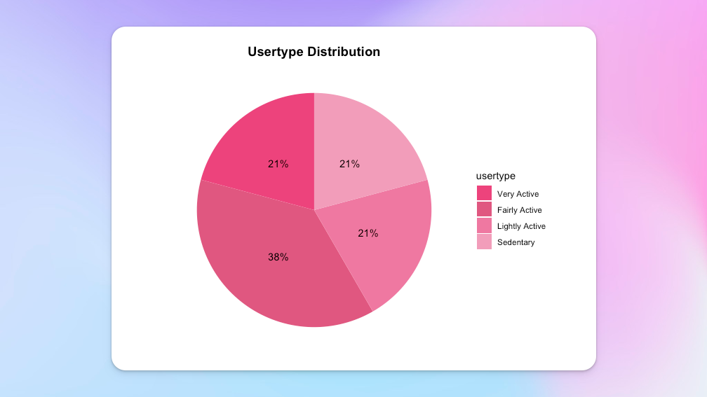
- Majority of the users are “Fairly Active.”
Calculate average steps walked and minutes slept by weekday
weekday_steps_and_sleep <- daily_activity_and_sleep %>%
  mutate(weekday = weekdays(date))

weekday_steps_and_sleep$weekday <- ordered(weekday_steps_and_sleep$weekday, levels = c("Monday", "Tuesday", "Wednesday", "Thursday", "Friday", "Saturday", "Sunday"))

weekday_steps_and_sleep <- weekday_steps_and_sleep %>%
  group_by(weekday) %>%
  summarise(daily_steps = mean(TotalSteps), daily_sleep = mean(TotalMinutesAsleep))

head(weekday_steps_and_sleep, 7)
Console output
# A tibble: 7 × 3
  **weekday   daily_steps daily_sleep**
    <ord>         <dbl>       <dbl>
1 Monday           9273         420
2 Tuesday          9183         405
3 Wednesday        8023         435
4 Thursday         8184         401
5 Friday           7901         405
6 Saturday         9871         419
7 Sunday           7298         453
Visualise weekly daily steps
ggplot(weekday_steps_and_sleep) +
  geom_col(aes(weekday, daily_steps), fill = "#ff7aa2") +
  geom_hline(yintercept = 7500) +
  labs(title =  "Weekly daily steps", x = "", y = "") +
  theme(axis.text.x = element_text(angle = 45, vjust = 0.5, hjust = 1)) +
  theme_bw()
Console output
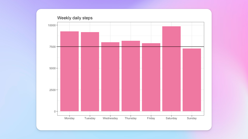
- All users are walking more than the recommended steps of 7,500.
- Saturday is the most active day with nearly 10,000 daily steps.
- Sunday is the least active day with below the recommended daily steps.
Visualise Weekly minutes slept
ggplot(weekday_steps_and_sleep, aes(weekday, daily_sleep)) +
  geom_col(fill = "#ff7aa2") +
  geom_hline(yintercept = 405) +
  labs(title = "Weekly minutes slept", x = "", y = "") +
  theme(axis.title.x = element_text(angle = 45, vjust = 0.5, hjust = 1)) +
  theme_bw()
Console output
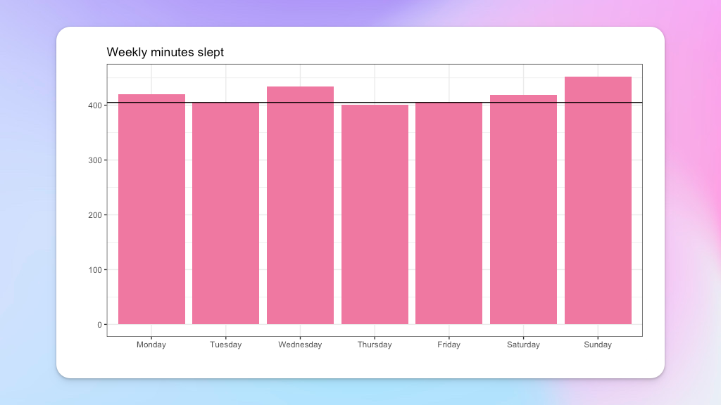
- Users are sleeping the recommended hours apart from Thursday.
- Users are sleeping the most on Sundays.
Calculate hourly steps
hourly_steps <- hourly_steps %>%
  separate(date_time, into = c("date", "time"), sep = " ") %>%
  mutate(date = ymd(date))

head(hourly_steps)
Console output
# A tibble: 6 × 4
Id       date     time StepTotal
1 1503960366 2016-04-12 00:00:00       373
2 1503960366 2016-04-12 01:00:00       160
3 1503960366 2016-04-12 02:00:00       151
4 1503960366 2016-04-12 03:00:00         0
5 1503960366 2016-04-12 04:00:00         0
6 1503960366 2016-04-12 05:00:00         0
Visualise Hourly Steps of the Day
hourly_steps %>%
  group_by(time) %>%
  summarise(average_steps = mean(StepTotal)) %>%
  ggplot() +
  theme_bw() +
  geom_col(mapping = aes(x = time, y = average_steps, fill = average_steps)) +
  labs(title = "Hourly steps of the day", x = "", y = "") +
  scale_fill_gradient(low = "lightpink", high = "#ff477e") +
  theme(axis.title.x = element_text(angle = 90, vjust = 0.5, hjust = 1))
Console output
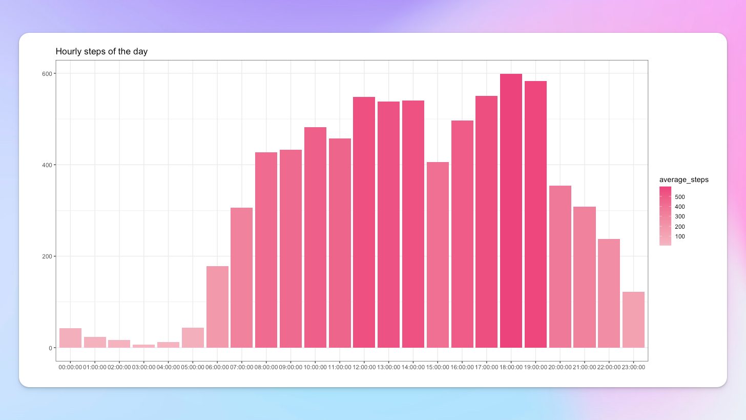
- Low steps from midnight until 6am as it is sleeping hours.
- Steps gradually increase from 7am onwards.
- Steps peak around 12pm until 2pm during lunch hours and again at 5pm until 7pm.
Daily Steps vs Minutes Slept correlation
ggplot(daily_activity_and_sleep, aes(x = TotalSteps, y = TotalMinutesAsleep)) +
  geom_jitter() +
  geom_smooth(colour = "#ff477e") +
  labs(title =  "Daily steps Vs Minutes slept", x = "Daily steps", y = "Minutes slept") +
  theme(panel.background = element_blank(), plot.title = element_text(size = 14))
Console output
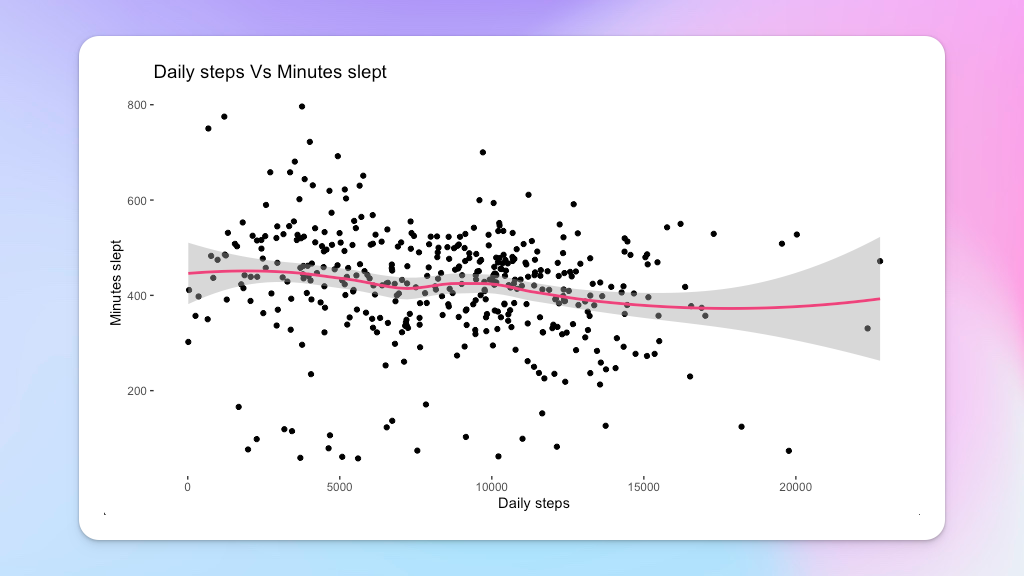
- There is no correlation between daily steps and the minutes users sleep.
- The amount of steps a user takes does not affect their sleeping pattern.
Daily Steps vs Calories correlation
ggplot(daily_activity_and_sleep, aes(x = TotalSteps, y = Calories)) +
  geom_jitter() +
  geom_smooth(colour = "#ff477e") +
  labs(title = "Daily steps Vs Calories", x = "Daily steps", y = "Calories") +
  theme(panel.background = element_blank(), plot.title = element_text(size = 14))
Console output
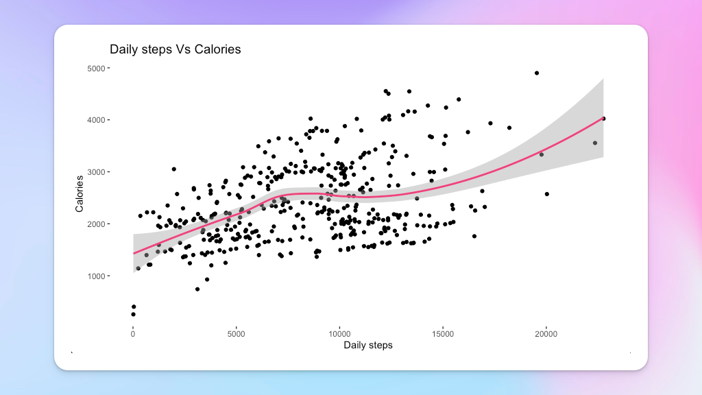
- There is a positive correlation between daily steps and the calories burnt.
- The more steps users take, the more calories they will burn.
Calculate number of daily use
daily_use <- daily_activity_and_sleep %>%
  group_by(Id) %>%
  summarise(days_used = sum(n())) %>%
  mutate(usage = case_when(
    days_used >= 1 & days_used <= 10 ~ "Low use",
    days_used >= 11 & days_used <= 20 ~ "Moderate use",
    days_used >= 21 & days_used <= 31 ~ "High use",))

head(daily_use,7)
Console output
# A tibble: 7 × 3
          **Id days_used usage**
       <dbl>     <int> <chr>
1 1503960366        25 High use
2 1644430081         4 Low use
3 1844505072         3 Low use
4 1927972279         5 Low use
5 2026352035        28 High use
6 2320127002         1 Low use
7 2347167796        15 Moderate use
Calculate daily use percentage
daily_use_percent <- daily_use %>%
  group_by(usage) %>%
  summarise(total = n()) %>%
  mutate(totals = sum(total)) %>%
  group_by(usage) %>%
  summarise(total_percent = total / totals) %>%
  mutate(labels = scales::percent(total_percent))

daily_use_percent$usage <- factor(daily_use_percent$usage, levels = c ("High use", "Moderate use", "Low use"))

head(daily_use_percent)
Console output
# A tibble: 3 × 3
  **usage        total_percent labels**
  <fct>                <dbl>  <chr>
1 High use             0.5      50%
2 Low use              0.375    38%
3 Moderate use         0.125    12%
Visualise daily use percentage
This will calculate the number of users using their smart devices.
daily_use_percent %>%
  ggplot(aes(x = "", y = total_percent, fill = usage)) +
  geom_bar(stat = "identity", width = 1) +
  coord_polar("y", start = 0) +
  theme_minimal() +
  theme(axis.title.x = element_blank(),
        axis.title.y = element_blank(),
        panel.border = element_blank(),
        panel.grid = element_blank(),
        axis.ticks = element_blank(),
        axis.text.x = element_blank(),
        plot.title = element_text(hjust = 0.5, size = 14, face = "bold")) +
  geom_text(aes(label = labels), position = position_stack(vjust = 0.5)) +
  scale_fill_manual(values = c ("#ff477e","#ff7aa2", "#ff9ebb"),
                    labels = c("High use - 21 to 31 days", "Moderate use - 11 to 20 days", "Low use - 1 to 10 days")) +
  labs(title = "Daily smart device use")
Console output
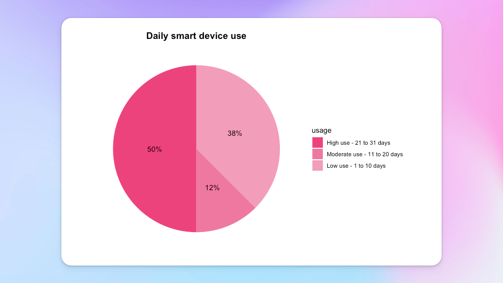
- Majority of the users are highly active on their smart devices and use it between 21 to 31 days.
- 12% of users use their smart devices between 11 to 20 days.
- More than 30% of users rarely use their smart devices, ranging from 1 to 10 days.
Merge daily activity and daily use
This will determine how often users wear their smart devices.
daily_use_and_activity <- merge(daily_activity, daily_use, by = c("Id"))

head(daily_use_and_activity)
Console output
Id                 date TotalSteps TotalDistance TrackerDistance LoggedActivitiesDistance VeryActiveDistance ModeratelyActiveDistance LightActiveDistance SedentaryActiveDistance
1 1503960366 2016-05-07      11992          7.71            7.71                        0               2.46                     2.12                3.13                       0
2 1503960366 2016-05-06      12159          8.03            8.03                        0               1.97                     0.25                5.81                       0
3 1503960366 2016-05-01      10602          6.81            6.81                        0               2.29                     1.60                2.92                       0
4 1503960366 2016-04-30      14673          9.25            9.25                        0               3.56                     1.42                4.27                       0
5 1503960366 2016-04-12      13162          8.50            8.50                        0               1.88                     0.55                6.06                       0
6 1503960366 2016-04-13      10735          6.97            6.97                        0               1.57                     0.69                4.71                       0
  VeryActiveMinutes FairlyActiveMinutes LightlyActiveMinutes SedentaryMinutes Calories days_used    usage
1                37                  46                  175              833     1821        25 High use
2                24                   6                  289              754     1896        25 High use
3                33                  35                  246              730     1820        25 High use
4                52                  34                  217              712     1947        25 High use
5                25                  13                  328              728     1985        25 High use
6                21                  19                  217              776     1797        25 High use
Calculate and group device usage in minutes
Here, another data frame was created to categorise the time period the users wear their smart devices.
minutes_device_worn <- daily_use_and_activity %>%
  mutate(total_minutes_wearing = VeryActiveMinutes + FairlyActiveMinutes + LightlyActiveMinutes + SedentaryMinutes) %>%
  mutate(percent_minutes_wearing = (total_minutes_wearing / 1440) * 100) %>%
  mutate(wearing = case_when(
    percent_minutes_wearing == 100 ~ "All day",
    percent_minutes_wearing < 100 & percent_minutes_wearing >= 50 ~ "More than half day",
    percent_minutes_wearing < 50 & percent_minutes_wearing > 0 ~ "Less than half day"))

head(minutes_device_worn)
Console output
**Id                 date TotalSteps TotalDistance TrackerDistance LoggedActivitiesDistance VeryActiveDistance ModeratelyActiveDistance LightActiveDistance SedentaryActiveDistance**
1 1503960366 2016-05-07      11992          7.71            7.71                        0               2.46                     2.12                3.13                       0
2 1503960366 2016-05-06      12159          8.03            8.03                        0               1.97                     0.25                5.81                       0
3 1503960366 2016-05-01      10602          6.81            6.81                        0               2.29                     1.60                2.92                       0
4 1503960366 2016-04-30      14673          9.25            9.25                        0               3.56                     1.42                4.27                       0
5 1503960366 2016-04-12      13162          8.50            8.50                        0               1.88                     0.55                6.06                       0
6 1503960366 2016-04-13      10735          6.97            6.97                        0               1.57                     0.69                4.71                       0
  **VeryActiveMinutes FairlyActiveMinutes LightlyActiveMinutes SedentaryMinutes Calories days_used    usage total_minutes_wearing percent_minutes_wearing            wearing**
1                37                  46                  175              833     1821        25 High use                  1091                75.76389 More than half day
2                24                   6                  289              754     1896        25 High use                  1073                74.51389 More than half day
3                33                  35                  246              730     1820        25 High use                  1044                72.50000 More than half day
4                52                  34                  217              712     1947        25 High use                  1015                70.48611 More than half day
5                25                  13                  328              728     1985        25 High use                  1094                75.97222 More than half day
6                21                  19                  217              776     1797        25 High use                  1033                71.73611 More than half day
Calculate device usage percentage
This data frame will illustrate the total number of users and the percentage of minutes they wore their devices for.
minutes_worn_percent <- minutes_device_worn %>%
  group_by(wearing) %>%
  summarise(total = n()) %>%
  mutate(totals = sum(total)) %>%
  group_by(wearing) %>%
  summarise(total_percent = total / totals) %>%
  mutate(labels = scales:: percent(total_percent))

head(minutes_worn_percent)
Console output
# A tibble: 3 × 3
  **wearing            total_percent labels**
  <chr>                      <dbl>  <chr>
1 All day                   0.365     36%
2 Less than half day        0.0351     4%
3 More than half day        0.600     60%
The next calculations will create three more data frames which will be filtered by the daily users category. This will then be able to differentiate the daily use and time use.
Calculate device usage by “High use” filter
minutes_worn_high_use <- minutes_device_worn %>%
  filter(usage == "High use") %>%
  group_by(wearing) %>%
  summarise(total = n()) %>%
  mutate(totals = sum(total)) %>%
  group_by(wearing) %>%
  summarise(total_percent = total / totals) %>%
  mutate(labels = scales::percent(total_percent))

head(minutes_worn_high_use)
Console output
# A tibble: 3 × 3
  **wearing            total_percent labels**
  <chr>                      <dbl>  <chr>
1 All day                   0.0676   6.8%
2 Less than half day        0.0432   4.3%
3 More than half day        0.889   88.9%
Calculate device usage by “Moderate use” filter
minutes_worn_mod_use <- minutes_device_worn %>%
  filter(usage == "Moderate use") %>%
  group_by(wearing) %>%
  summarise(total = n()) %>%
  mutate(totals = sum(total)) %>%
  group_by(wearing) %>%
  summarise(total_percent = total / totals) %>%
  mutate(labels = scales::percent(total_percent))

head(minutes_worn_mod_use)
Console output
# A tibble: 3 × 3
  **wearing            total_percent labels**
  <chr>                      <dbl> <chr>
1 All day                    0.267 27%
2 Less than half day         0.04  4%
3 More than half day         0.693 69%
Calculate device usage by “Low use” filter
minutes_worn_low_use <- minutes_device_worn %>%
  filter(usage == "Low use") %>%
  group_by(wearing) %>%
  summarise(total = n()) %>%
  mutate(totals = sum(total)) %>%
  group_by(wearing) %>%
  summarise(total_percent = total / totals) %>%
  mutate(labels = scales::percent(total_percent))

head(minutes_worn_low_use)
Console output
# A tibble: 3 × 3
  **wearing            total_percent labels**
  <chr>                      <dbl>  <chr>
1 All day                   0.802     80%
2 Less than half day        0.0224     2%
3 More than half day        0.175     18%
Visualise time worn per day
ggplot(minutes_worn_percent, aes(x="",y=total_percent, fill=wearing)) +
  geom_bar(stat = "identity", width = 1) +
  coord_polar("y", start = 0) +
  theme_minimal() +
  theme(axis.title.x= element_blank(),
        axis.title.y = element_blank(),
        panel.border = element_blank(),
        panel.grid = element_blank(),
        axis.ticks = element_blank(),
        axis.text.x = element_blank(),
        plot.title = element_text(hjust = 0.5, size = 14, face = "bold"),
        plot.subtitle = element_text(hjust = 0.5)) +
  scale_fill_manual(values = c("#ff477e","#ff7aa2", "#ff9ebb")) +
  geom_text(aes(label = labels),
            position = position_stack(vjust = 0.5), size = 3.5) +
  labs(title="Time worn per day", subtitle = "Total Users")
Console output
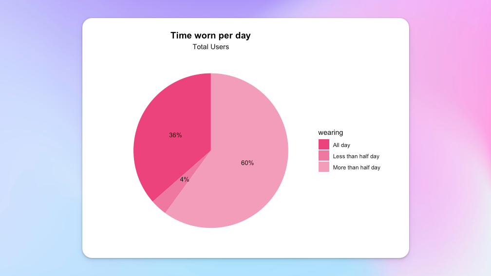
- More than 30% of users wear their devices “All day.”
- 4% of users wear their devices “Less than half a day.”
- Majority of the users wear their devices “More than half a day.”
Visualise time worn per day by “High use” users
ggplot(minutes_worn_high_use, aes(x="",y=total_percent, fill=wearing)) +
  geom_bar(stat = "identity", width = 1) +
  coord_polar("y", start = 0) +
  theme_minimal() +
  theme(axis.title.x= element_blank(),
        axis.title.y = element_blank(),
        panel.border = element_blank(),
        panel.grid = element_blank(),
        axis.ticks = element_blank(),
        axis.text.x = element_blank(),
        plot.title = element_text(hjust = 0.5, size = 14, face = "bold"),
        plot.subtitle = element_text(hjust = 0.5),
        legend.position = "none") +
  scale_fill_manual(values = c("#ff477e","#ff7aa2", "#ff9ebb")) +
  geom_text_repel(aes(label = labels),
                  position = position_stack(vjust = 0.5), size = 3) +
  labs(title="Time worn per day", subtitle = "High use users")
Console output 
- 6.8% of users wore and used their devices “All day”.
- 88.9% of users wore and used their devices “More than half a day.”
- 4.3% of users wore and used their devices “Less than half a day.”
Visualise time worn per day by “Moderate use” users
ggplot(minutes_worn_mod_use, aes(x="",y=total_percent, fill=wearing)) +
  geom_bar(stat = "identity", width = 1) +
  coord_polar("y", start = 0) +
  theme_minimal() +
  theme(axis.title.x= element_blank(),
        axis.title.y = element_blank(),
        panel.border = element_blank(),
        panel.grid = element_blank(),
        axis.ticks = element_blank(),
        axis.text.x = element_blank(),
        plot.title = element_text(hjust = 0.5, size = 14, face = "bold"),
        plot.subtitle = element_text(hjust = 0.5),
        legend.position = "none") +
  scale_fill_manual(values = c("#ff477e","#ff7aa2", "#ff9ebb")) +
  geom_text(aes(label = labels),
            position = position_stack(vjust = 0.5), size = 3) +
  labs(title="Time worn per day", subtitle = "Moderate use users")
Console output 
- 27% of users used their smart devices for the entire day.
- 69% of users used their smart devices for “More than half a day.”
- 4% of users rarely use their smart devices.
Visualise time worn per day by “Low use” users
ggplot(minutes_worn_low_use, aes(x="",y=total_percent, fill=wearing)) +
  geom_bar(stat = "identity", width = 1) +
  coord_polar("y", start = 0) +
  theme_minimal() +
  theme(axis.title.x= element_blank(),
        axis.title.y = element_blank(),
        panel.border = element_blank(),
        panel.grid = element_blank(),
        axis.ticks = element_blank(),
        axis.text.x = element_blank(),
        plot.title = element_text(hjust = 0.5, size = 14, face = "bold"),
        plot.subtitle = element_text(hjust = 0.5),
        legend.position = "none") +
  scale_fill_manual(values = c("#ff477e","#ff7aa2", "#ff9ebb")) +
  geom_text(aes(label = labels),
            position = position_stack(vjust = 0.5), size = 3) +
  labs(title = "Time worn per day", subtitle = "Low use users")
Console output 
- 80% of users use their smart devices for the entire day.
- 18% of users use their smart devices for “More than half a day.”
- 2% of users rarely use their smart devices.
Act
This section will cover the recommendations based on the information and findings discovered. Bellabeat needs to focus on tracking their own data to respond and assist to their mission and business task.
In order to come up with the correct marketing strategy for it’s products Bellabeat could create the following:
- Calorie counter: A counter could encourage a user to use the app and smart device a lot more with an appealing designed interface which displays the number of calories that are burnt during use. To further improve user motivation, customisable features could be added to allow users to be in control of their apps and create “goals”.
- Sleep log: Although, the sampled users have consistent sleeping patterns, some users may want to track their sleeping habits. This feature could boost Bellabeat app use a lot, as it would enable to recording of number of wakes during the night, sleep quality, and total awake time in bed. With this data, the app could recommend the user a certain time to be in bed by and this could be customisable by the user.
- Push notifications: As discovered from the findings, some users are not walking the recommended steps and not sleeping the recommended hours. In order to combat this, Bellabeat could push notifications to users if they are low in steps for the day, close to their “goals” or if it’s nearing their bed time. This would motivate users to make more use of their apps and smart devices.
- Daily, weekly and monthly achievements: The Bellabeat app could provide users with insightful and interactive reports based on their steps, calories burnt, and sleeping habits. Badges and messages could be sent to users to motivate them and encourage them to continue with their good habits.
- Daily health words of wisdom and improvements: Bellabeat could push daily words of wisdom on health in the app to motivate and encourage their users to use the app or their smart devices. This can also include tips or improvements on the users overall performance to get them to achieve their “goals”.
- Discounts on other products: Special discounts on different Bellabeat products can be offered to users in order to retain and keep them motivated. This will act as an incentive and incline users to purchase more products and stay active. Moreover, discounts can be given on Bellabeat’s premium membership as well.
No further recommendation was made to Bellabeat as the data set could have been biased as it was limited due to having a very small sample size and a lack in user demographic information such as age. Having this information available could have been extremely useful in gaining movement insights and trends of women in different age groups.